


2. 江南大学物联网工程学院, 江苏 无锡 214122
2. School of Internet of Things Engineering, Jiangnan University, Wuxi 214122, China
1 引言
系统辨识是由系统的输入输出的时间函数来确定描述系统行为的数学模型[1, 2]. 系统辨识为了估计表征系统的未知参数建立一个能模仿真实系统行为的模型,预测出系统在下一时刻的输入和输出值及设计控制器[3, 4]. 分解的思想在3阶段辨识方法中的运用将是一个突破性的创新[5, 6]. 从分解思想出发,运用3阶段辨识原理结合最小二乘辨识算法对两输入单输出输出误差类模型进行辨识[7, 8],并运用Matlab等仿真工具证明本算法的有效性. 本课题的研究首先是从分解的思想出发,结合递阶辨识原理和递推最小二乘算法[9, 10],利用计算机仿真说明分解递推最小二乘(DRLS)算法能得到高精度的参数估计.
对于输出误差类模型,目前已经有很多方法估计其参数,如偏差补偿最小二乘法[11]、 辅助模型法[12]和迭代辨识方法[13]等,但当系统维数较大时,这些传统的辨识方法参数估计过程中的计算量较大,其每次递推中迭代算法的巨大计算量使得一般的工业计算机无法实现实时响应[14, 15, 16, 17]. 本文研究的分解递推方法,将系统分解成3个子系统,然后分别估计各个子系统的参数[18],最后协调各子系统的辨识结果,减少了计算中向量的维数,减小了求逆运算的计算量,辨识过程的整体计算量会大大地降低[19, 20],提高计算效率.
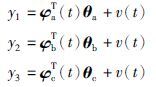
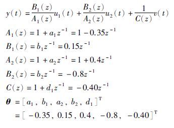
2 系统描述与问题构成设两输入单输出输出误差自回归模型描述为
设阶次n和nc已知且当t≤0时,y(t)=0,ui(t)=0和v(t)=0. 定义系统真实输出xi(t)和噪声模型输出w(t)分别为
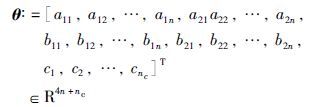
定义参数向量:
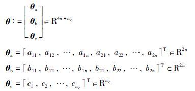
定义参数向量:
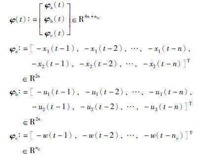
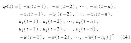
定义信息向量:
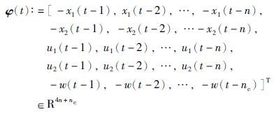
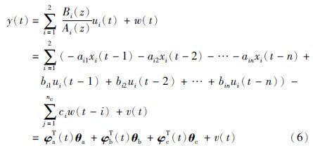
方程(6)可以写成:
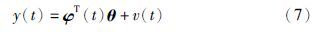
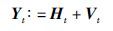
定义:
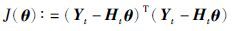
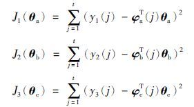
根据最小二乘原理,定义二次准则函数:
定义3个虚拟输出变量:
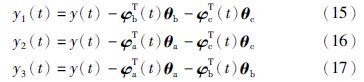
系统(6)可以分解为下列3个子系统模型:
这3个子系统包含了参数向量θa、 θb和θc定义的3个准则函数:
令J1(θa)、 J2(θb)和J3(θc)分别关于参数向量θa、 θb和θc的偏导数为0,令R4n+nc
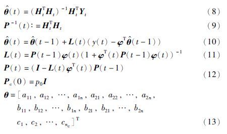
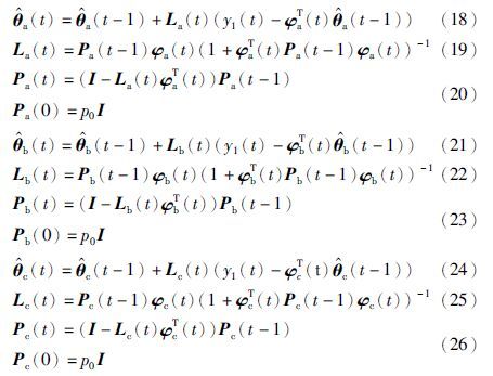
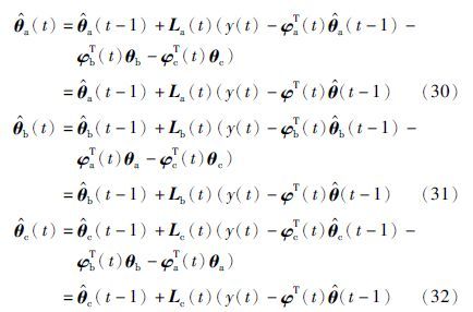
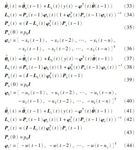
在t时刻的估计,由以上3个公式可以得到下列分解递推最小二乘算法:
将式(15)~(17)分别代入式(18)、 式(21)和式(24)得
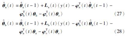
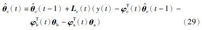
困难在于式(27)~(29)右边分别包含了未知参数向量θa、 θb和θc,使得这个递推算法不能实现,解决的方法是: 式(27)~(29)中未知参数向量θa、 θb和θc分别用其在时刻t-1的估计 和
和 代替,得到
代替,得到
分解递推最小二乘算法(33)、 (34)来计算参数估计向量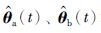 和
和 的步骤如下:
(1) 令t=1,置初值Pa(0)=p0I,Pb(0)=p0I,Pc(0)=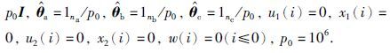
(2) 收集输入输出数据ui、 xi和wi,由式(36)、 式(40)和式(44)构成信息向量φa(t)、 φb(t)和φc(t).
(3) 采用式(34)、 式(38)和式(42)分别计算增益向量La(t)、 Lb(t)和Lc(t),采用式(35)、 式(39)和式(43)分别计算协方差阵Pa(t)、 Pb(t)和Pc(t).
(4) 由式(33)、 式(37)和式(41)分别刷新参数估计向量 和
和 .
.
(5) t=t+1,转到步骤(2),继续进行递推运算.
5 仿真实验下面通过2个例子来说明提出算法的有效性.
例1 考虑下面的TISO-OE模型:
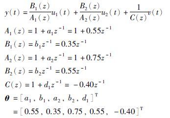
仿真时,{u1(t)}和{u2(t)}两个不相关的持续激励信号序列的均值为零和单位方差; {v(t)}为均值为零、 方差为σ12=0.102和σ22=0.502的白噪声向量序列. 应用提出的算法估计这个系统的参数,不同数据长度下参数估计和估计误差如表 1~4所示,参数估计误差 随t变化曲线如图 1~4所示.
| 算法 | t | a1 | a2 | b1 | b2 | d1 | δ /% |
| DRLS | 100 | 0.528 21 | 0.712 94 | 0.343 89 | 0.611 37 | -0.469 38 | 9.687 27 |
| 200 | 0.551 19 | 0.745 28 | 0.354 64 | 0.592 74 | -0.435 95 | 5.424 88 | |
| 500 | 0.567 85 | 0.768 52 | 0.372 58 | 0.570 47 | -0.413 99 | 4.098 66 | |
| 1 000 | 0.578 69 | 0.759 69 | 0.341 05 | 0.557 41 | -0.379 95 | 3.597 59 | |
| 2 000 | 0.557 91 | 0.748 70 | 0.341 86 | 0.557 00 | -0.398 20 | 1.111 49 | |
| 3 000 | 0.552 54 | 0.752 85 | 0.340 73 | 0.554 87 | -0.391 92 | 1.039 68 | |
| RLS | 100 | 0.672 64 | 0.761 07 | 0.316 28 | 0.530 33 | -0.183 88 | 19.904 36 |
| 200 | 0.621 38 | 0.747 39 | 0.349 55 | 0.537 75 | -0.288 62 | 11.471 24 | |
| 500 | 0.603 34 | 0.763 22 | 0.375 62 | 0.560 37 | -0.310 44 | 9.009 60 | |
| 1 000 | 0.596 90 | 0.759 96 | 0.336 67 | 0.552 69 | -0.321 16 | 7.614 80 | |
| 2 000 | 0.569 23 | 0.742 19 | 0.341 34 | 0.551 36 | -0.383 04 | 2.603 67 | |
| 3 000 | 0.557 26 | 0.747 03 | 0.338 71 | 0.553 02 | -0.385 13 | 1.593 80 | |
| 真值 | 0.550 00 | 0.750 00 | 0.350 00 | 0.550 00 | -0.400 00 |
| 算法 | t | a1 | a2 | b1 | b2 | d1 | δ /% |
| DRLS | 100 | 0.526 55 | 0.746 56 | 0.373 11 | 0.540 56 | -0.408 64 | 2.749 92 |
| 200 | 0.558 15 | 0.763 72 | 0.360 24 | 0.550 63 | -0.371 67 | 2.804 47 | |
| 500 | 0.548 23 | 0.761 26 | 0.357 92 | 0.550 54 | -0.403 38 | 1.230 58 | |
| 1 000 | 0.547 67 | 0.755 41 | 0.355 56 | 0.551 66 | -0.385 65 | 1.222 23 | |
| 2 000 | 0.548 76 | 0.754 25 | 0.354 92 | 0.549 45 | -0.396 73 | 0.717 39 | |
| 3 000 | 0.548 46 | 0.752 41 | 0.353 13 | 0.549 86 | -0.403 61 | 0.489 97 | |
| RLS | 100 | 0.563 18 | 0.772 94 | 0.359 72 | 0.539 80 | -0.150 20 | 18.724 92 |
| 200 | 0.566 26 | 0.773 79 | 0.351 18 | 0.543 19 | -0.188 43 | 16.120 73 | |
| 500 | 0.552 36 | 0.764 49 | 0.354 76 | 0.547 73 | -0.334 07 | 4.850 29 | |
| 1 000 | 0.553 12 | 0.758 25 | 0.353 60 | 0.551 18 | -0.344 04 | 4.237 24 | |
| 2 000 | 0.552 35 | 0.756 12 | 0.354 11 | 0.548 70 | -0.378 28 | 1.750 57 | |
| 3 000 | 0.551 46 | 0.753 75 | 0.352 27 | 0.549 68 | -0.389 51 | 0.931 46 | |
| 真值 | 0.550 00 | 0.750 00 | 0.350 00 | 0.550 00 | -0.400 00 |
| 算法 | t | a1 | a2 | b1 | b2 | d1 | δ /% |
| DRLS | 100 | -0.193 35 | 0.803 84 | 0.227 48 | -0.836 85 | -0.087 24 | 37.830 17 |
| 200 | -0.219 36 | 0.680 96 | 0.160 25 | -0.832 13 | -0.139 20 | 31.510 57 | |
| 500 | -0.290 59 | 0.623 81 | 0.161 58 | -0.812 05 | -0.309 34 | 11.158 67 | |
| 1 000 | -0.337 96 | 0.506 25 | 0.153 91 | -0.792 48 | -0.345 70 | 5.988 71 | |
| 2 000 | -0.325 07 | 0.453 91 | 0.161 66 | -0.806 00 | -0.362 55 | 4.892 16 | |
| 3 000 | -0.328 04 | 0.409 62 | 0.158 57 | -0.801 06 | -0.376 13 | 3.445 58 | |
| RLS | 100 | -0.204 07 | 0.873 44 | 0.193 35 | -0.837 70 | -0.093 28 | 35.437 43 |
| 200 | -0.228 17 | 0.751 63 | 0.176 83 | -0.803 76 | -0.085 93 | 34.765 60 | |
| 500 | -0.243 84 | 0.645 24 | 0.165 61 | -0.809 88 | -0.204 92 | 22.925 49 | |
| 1 000 | -0.294 27 | 0.610 29 | 0.155 52 | -0.804 10 | -0.236 10 | 17.821 93 | |
| 2 000 | -0.290 30 | 0.459 20 | 0.158 24 | -0.810 86 | -0.288 88 | 13.051 76 | |
| 3 000 | -0.296 45 | 0.410 38 | 0.161 16 | -0.807 46 | -0.314 08 | 10.505 20 | |
| 真值 | 0.550 00 | 0.750 00 | 0.350 00 | 0.550 00 | -0.400 00 |
| 算法 | t | a1 | a2 | b1 | b2 | d1 | δ /% |
| DRLS | 100 | -0.323 20 | 0.673 52 | 0.165 49 | -0.806 95 | -0.137 48 | 28.281 36 |
| 200 | -0.327 49 | 0.590 38 | 0.152 02 | -0.806 69 | -0.186 86 | 23.221 58 | |
| 500 | -0.339 80 | 0.501 03 | 0.152 39 | -0.802 59 | -0.308 90 | 9.171 54 | |
| 1 000 | -0.348 60 | 0.473 02 | 0.150 79 | -0.798 60 | -0.330 81 | 7.270 75 | |
| 2 000 | -0.345 46 | 0.416 2 | 0.152 30 | -0.801 23 | -0.368 13 | 3.320 77 | |
| 3 000 | -0.345 85 | 0.390 71 | 0.151 67 | -0.800 23 | -0.383 01 | 1.805 41 | |
| RLS | 100 | -0.325 09 | 0.730 29 | 0.162 51 | -0.797 76 | -0.058 06 | 35.292 35 |
| 200 | -0.330 13 | 0.629 01 | 0.156 62 | -0.796 67 | -0.073 41 | 33.666 56 | |
| 500 | -0.336 74 | 0.557 28 | 0.153 07 | -0.799 56 | -0.161 12 | 24.612 86 | |
| 1 000 | -0.345 63 | 0.539 27 | 0.151 10 | -0.799 17 | -0.218 68 | 18.658 63 | |
| 2 000 | -0.343 02 | 0.439 93 | 0.151 58 | -0.800 78 | -0.285 83 | 11.768 00 | |
| 3 000 | -0.343 84 | 0.409 93 | 0.152 05 | -0.800 29 | -0.317 99 | 8.462 38 | |
| 真值 | 0.550 00 | 0.750 00 | 0.350 00 | 0.550 00 | -0.400 00 |

|
| 图 1 DRLS和RLS参数估计误差σ随t变化曲线(σ2=0.502) Fig. 1 The estimation errors σ of DRLS and RLS with the changes of t (σ2=0.502) |

|
| 图 2 DRLS和RLS参数估计误差σ随t变化曲线(σ2=0.102) Fig. 2 The estimation errors σ of DRLS and RLS with the changes of t (σ2=0.102) |

|
| 图 3 DRLS和RLS参数估计误差σ随t变化曲线(σ2=0.502) Fig. 3 The estimation errors σ of DRLS and RLS with the changes of t (σ2=0.502) |

|
| 图 4 DRLS和RLS参数估计误差σ随t变化曲线(σ2=0.102) Fig. 4 The estimation errors σ of DRLS and RLS with the changes of t (σ2=0.102) |
从图 1~4和表 1~4可以看出: 随着数据长度的增加,分解递推最小二乘算法参数估计逐渐收敛于真参数; 参数估计误差越来越小,估计精度是令人满意的且其计算量小.
表 5比较了RLS和DRLS算法在每一步递推计算中的乘法次数和加法次数,方括号中的次数表示系统输入数和阶次在每一步中的递推计算次数. 从表 5可以看出,DRLS算法明显比RLS小.
| 变量 | 乘法次数 | 加法次数 |
| RLS | 4n2+5n[125] | 4n(n+1)[104] |
| DRLS | 4[na12+na22+nb12+nb22+nc2]+5n[45] | 4[na12+na22+nb12+nb22+nc2]+2n[31] |
例2 考虑下面的TISO-OE模型:
本文研究了基于分解的识别思想结合递推最小二乘算法的两输入单输出输出误差模型,比较了DRLS和RLS算法的有效性. 仿真结果表明,与RLS相比,该算法具有计算量小的优点. 本文中的识别方法可用于估计系统参数来设计过滤器或反馈控制律的不确定系统或多速率系统. 本文的仿真实验只在数据上表明了提出算法的收敛性,没有给出严格的数学证明,这也是许多辨识算法的难点和不足之处.
| [1] | 丁锋. 系统辨识新论[M]. 北京: 科学出版社, 2013. Ding F. A new system identification[M]. Beijing: Science Press, 2013. |
| [2] | 于一发, 张大庆, 张波, 等. 基于Tikhonov正则化的模糊系统辨识方法[J]. 信息与控制, 2014, 43(4): 447-450, 456. Yu Y F, Zhang D Q, Zhang B, et al. Fuzzy model identification method based on Tikhonov regularization[J]. Information and Control, 2014, 43(4): 447-450, 456. |
| [3] | 李晓华, 李军. 基于ESN网络的连续搅拌反应釜(CSTR)辨识[J]. 信息与控制, 2014, 43(2): 223-228. Li X H, Li J. Identification of continuous stirred tank reactor based on echo state network[J]. Information and Control, 2014, 43(2): 223-228. |
| [4] | 丁锋, 杨家本. 大系统的递阶辨识[J]. 自动化学报, 1999, 25(5): 647-654. Ding F, Yang J B. Hierarchical identification of large systems[J]. Automation, 1999, 25(5): 647-654. |
| [5] | Shi Y, Yu B. Output feedback stabilization of networked control systems with random delays modeled by Markov chains[J]. IEEE Transactions on Automatic Control, 2009, 54(7): 1668-1674. |
| [6] | Shi Y, Huang J, Yu B. Robust tracking control of networked control systems: Application to a networked DC motor[J]. IEEE Transactions on Industrial Electronics, 2013, 60(12): 5864-5874. |
| [7] | Li H, Shi Y. Robust distributed model predictive control of constrained continuous-time nonlinear systems: A robustness constraint approach[J]. IEEE Transactions on Automatic Control, 2014, 59(6): 1673-1678. |
| [8] | Zhang W G. Decomposition based least squares iterative estimation for output error moving average systems[J]. Engineering Computations, 2014, 31(4): 709-725. |
| [9] | Voros J. Recursive identification of Hammerstein systems with discontinuous nonlinearities containing dead-zones[J]. IEEE Transactions on Automatic Control, 2004, 48(12): 2203-2206. |
| [10] | 王冬青. 基于辅助模型的递推增广最小二乘辨识方法[J]. 控制理论与应用, 2009, 26(1): 51-56. Wang D Q. Auxiliary model based the recursive extended least squares identification method[J]. Journal of Control Theory and Applications, 2009, 26(1): 51-56. |
| [11] | Voros J. Iterative algorithm for parameter identification of Hammerstein systems with two-segment nonlinearities[J]. IEEE Transactions on Automatic Control, 1999, 44(11): 2145-2149. |
| [12] | Kermani M M, Dehestani M. Solving the nonlinear equations for one-dimensional nano-sized model including Rydberg and Varshni potentials and Casimir force using the decomposition method[J]. Applied Mathematical Modelling, 2013, 37(5): 3399-3406. |
| [13] | 檀国节. 一种新的线性分布参数系统辨识方法[J]. 信息与控制, 1994, 23(4): 212-214, 222. Tan G J. A new methodfor parameter identification of linear distributed parameter systems[J]. Information and Control, 1994, 23(4): 212-214, 222. |
| [14] | Ding F, Duan H H. Two-stage parameter estimation algorithms for Box-Jenkins systems[J]. IET Signal Processing, 2013, 7(8): 646-654. |
| [15] | 杨慧中, 张勇. Box-Jenkins模型偏差补偿方法与其他辨识方法的比较[J]. 控制理论与应用, 2007, 24(2): 215-222. Yang H Z, Zhang Y. Comparison between Box-Jenkins model bias compensation method and other identification method[J]. Journal of Control Theory and Applications, 2007, 24(2): 215-222. |
| [16] | 汤笑笑, 李介谷. 基于小波神经网络的系统辨识方法[J]. 信息与控制, 1998, 27(4): 277-281, 288. Tang X X, Li J G. Wavelet neural networks based system identification[J]. Information and Control, 1998, 27(4): 277-281, 288. |
| [17] | 罗晓, 陈耀, 孙优贤. 基于小波变换的含噪系统辨识[J]. 信息与控制, 2003, 32(5): 467-470, 474. Luo X, Chen Y, Sun Y X. Noisy system identification based on wavelet[J]. Information and Control, 2003, 32(5): 467-470, 474. |
| [18] | Lu X L, Shi W L, Zhou W. Decomposition based least squares iterative estimation algorithm for two-input single-output output error systems[J]. Journal of the Franklin Institute, 2014, 315(12): 5511-5522. |
| [19] | Wang D Q. Input-output data filtering based recursive least squares parameter estimation for CARARMA systems[J]. Digital Signal Processing, 2010, 20(4): 991-999. |
| [20] | Bai E W. An optimal two-stage identification algorithm for Hammerstein-Wiener nonlinear systems[J]. Automatica, 1998, 34(3): 333-338. |